Introduction
Scientific computing has long faced a trade-off: high-level libraries offer convenience, rich syntax, and diverse data types that enable rapid prototyping, while low-level languages provide fine-grained control over memory management, enabling direct kernel and hardware-specific optimizations crucial for high performance.
In recent years, pairing Python interfaces with high-performance kernels in lower-level languages has emerged as a new scientific software design pattern (see: JAX, Numba, Taichi). The approach separates code semantics from compiler optimizations, and continued improvements in the latter are narrowing performance trade-offs. The success of this framework has encouraged more researchers to adopt high-level tooling, leading to development of domain-specific extensions in fields traditionally dominated by low-level libraries, such as molecular dynamics (MD), computational fluid dynamics (CFD), and finite element analysis (FEA).
As this paradigm continues to gain momentum, many new researchers have grown comfortable using these tools as black boxes. However, developing with both high-level and low-level mindsets need not be mutually exclusive. Understanding the architecture of high-level tools can significantly enhance our capabilities as scientific software developers. This architectural knowledge enables us to write more efficient code, leverage advanced features effectively, and diagnose performance bottlenecks with greater precision.
We'll take JAX as an example, exploring how insights into its internal workings can lead to more thoughtful algorithm design and implementation.
JAX's Execution Pipeline
While all high-level libraries ultimately execute as machine instructions, JAX distinguishes itself in its translation process. Libraries like NumPy already offer excellent performance for array operations by leveraging pre-compiled C and Fortran code. JAX takes this one step further by employing a compilation strategy that allows for optimization across operation boundaries and more effective use of hardware accelerators.
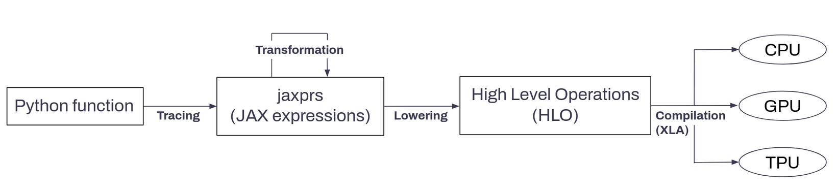
JAX achieves these optimizations through three key technologies:
1. Static Computation Tracing
When a function is first called, JAX creates a blueprint of its computational structure via tracing:
- Function inputs are replaced by
Tracerobjects, which hold only abstract information about the inputs (shape and data type), rather than their actual values. - Operations executed on the
Tracerobjects are intercepted (recorded) as a sequence of granular primitives (e.g.add,multiply,sin).
This process generates a jaxpr (JAX exPRession) - a static, intermediate representation of the function. Jaxprs are independent of specific input values, serving as the basis for JAX to transform (technology 2) and compile (technology 3) computations without re-executing the original Python code.
2. Composable Transformations
Transformations in JAX are higher order functions (they take functions as input and produce new, modified functions as output). Like creating recipe variations (e.g. a larger batch version, a calorie-reduced version, or an optimized quick-prep version), transformations of functions are what make JAX inherently versatile.
JAX's transformations work by reinterpreting the computational graph and jaxpr representation of the function generated during tracing. For example:
jax.grad(): Traces the function to a jaxpr, splits it into forward and backward passes, then uses primitive-specific transpose rules to propagate gradients via the chain rule.jax.vmap(): Rewrites each primitive in the jaxpr to handle additional batch dimensions. A batching rule is applied to each primitive to determine how to lift it to operate over additional axes.jax.jit(): (More detail in the next section). Just-in-time compiles the function by converting its jaxpr to optimized machine code. Compiled executables are cached based on argument shapes and types, enabling efficient reuse.
These transformations can be composed, creating a pipeline of modifications. For instance, we could differentiate a function, vectorize the resulting gradient computation, and then JIT-compile the vectorized gradient. This a key feature of JAX, allowing users to express complex operations concisely and efficiently.
3. Compilation and Caching
JAX leverages the XLA (Accelerated Linear Algebra) compiler to translate functions into highly optimized, low-level code for specific hardware targets. This is primarily achieved through JIT (Just-In-Time) compilation, though AOT (Ahead-Of-Time) compilation is also available.
In practice, JAX achieves this by lowering its jaxpr representation into XLA’s own intermediate representation, known as High-Level Operations (HLO). HLO provides a more explicit set of (hardware-specific) operations from which XLA can perform aggressive optimizations, such as operation fusion and memory layout transformations. The result is an optimized, hardware-specific executable.
For example, when jax.jit() is first called, JAX:
- Triggers additional tracing to lower the jaxpr into HLO.
- Compiles the HLO into an executable for a target architecture (CPU, GPU, or TPU)
- Caches the executable based on input shapes and data types. For subsequent calls with compatible inputs, JAX bypasses Python execution and directly runs the cached executable (i.e. transfers the inputs to the XLA device, executes the program, and returns the outputs).
There is, however, a trade-off between compilation time and execution time. JIT compilation can introduce latency on the first call, but this is usually amortized over multiple calls to the same function with similar inputs. For functions that are called infrequently or with highly variable input shapes, this compilation strategy introduces an overhead that could outweigh the performance benefits. In some situations AOT compilation may be preferable, where functions are compiled prior to execution time.
Jaxprs: Deciphering JAX's Computational Blueprint
All three technologies above speak the jaxpr language (see Figure 1). Although examining jaxprs alone may not fully reveal the optimizations performed by XLA in the final stages of the execution pipeline, understanding them provides insight into the assumptions JAX makes about your code. This knowledge may help us make informed adjustments, guiding JAX’s machinery to optimize for specific performance goals.
Conceptually, we can think of jaxprs as computational blueprints, composed of three main elements:
- Input binders: Typed variables representing function inputs.
- Equations: A sequence of primitive applications defining the computation.
- Output expressions: Specifying the function's results.
Formally, jaxprs are data structures represented like:
jaxpr ::= { lambda <binders>. let <eqns> in <outputs> }
binders ::= <var>:<type>, ...
eqns ::= <eqn>, ...
eqn ::= <outputs> = <primitive>[<params>] <inputs>
outputs ::= <var>, ...
inputs ::= <expr>, ...
expr ::= <var> | <literal>
where variables are typed using ShapedArray (encapsulating both shape and data type information) and literals represent constant values (typically scalars or small arrays).
Example: Feed Forward Layer
To illustrate the nuances of jaxpr generation, we'll look at three implementations of applying a simple feed forward layer to batched inputs (an exercise inspired by the following post):
- Standard Python loop (i.e. using native python control flow)
jax.lax.map(thejax.laxmodule houses JAX’s primitives that correspond closely to operations in XLA, withjax.lax.mapbeing the analogue for Python’s native map function)jax.vmap(i.e. vectorizing across batch dimension)
Examining the jaxpr generated by each implementation reveals JAX's distinct interpretations of batching, which in turn influences each is lowered into HLO and handled by XLA. Quantitatively speaking, this impacts both compilation and execution times, making it a key factor to consider for performance.
Here are the implementations:
import jax
import jax.numpy as jnp

# Simple feed forward layer
def layer_forward(params, x):
    w, b = params
    return jax.nn.relu(jnp.dot(w, x) + b)

# 1. Standard Python loop
def batch_forward_for_loop(params, batch):
    return jnp.array([layer_forward(params, x) for x in batch])

# 2. `jax.lax.map`
def batch_forward_lax_map(params, batch):
    return jax.lax.map(lambda x: layer_forward(params, x), batch)

# 3. `jax.vmap`
batch_forward_vmap = jax.vmap(layer_forward, in_axes=(None, 0))
1. Standard Python Loop
JAX describes the make_jaxpr transformation as a “pretty-printing” transformation, transforming a function into one that, given arguments, produces a jaxpr representation of itself. Printing is as simple as:
print(jax.make_jaxpr(batch_forward_for_loop)(params, x))For the standard Python loop, the resulting jaxpr is quite verbose. Its format resembles a mini functional programming language composed of various primitives. For example:
sliceandsqueezeoperations extract individual samples from the batch.dot_generalperforms the matrix multiplication between weights and input.addapplies the bias.custom_jvp_callencapsulates the ReLU activation, allowing for custom gradient definitions.broadcast_in_dimandconcatenateoperations reassemble the results into a batch.
In full:
let relu = { lambda ; a:f32[32]. let b:f32[32] = max a 0.0 in (b,) } in
{ lambda ; c:f32[32,64] d:f32[32] e:f32[2,64]. let
    f:f32[1,64] = slice[
      limit_indices=(1, 64)
      start_indices=(0, 0)
      strides=(1, 1)
    ] e
    g:f32[64] = squeeze[dimensions=(0,)] f
    h:f32[32] = dot_general[
      dimension_numbers=(([1], [0]), ([], []))
      preferred_element_type=float32
    ] c g
    i:f32[32] = add h d
    j:f32[32] = custom_jvp_call[
      call_jaxpr={ lambda ; k:f32[32]. let
          l:f32[32] = pjit[name=relu jaxpr=relu] k
        in (l,) }
      jvp_jaxpr_thunk=<function _memoize.<locals>.memoized at 0x75cab752a710>
      num_consts=0
      symbolic_zeros=False
    ] i
    m:f32[1,64] = slice[
      limit_indices=(2, 64)
      start_indices=(1, 0)
      strides=(1, 1)
    ] e
    n:f32[64] = squeeze[dimensions=(0,)] m
    o:f32[32] = dot_general[
      dimension_numbers=(([1], [0]), ([], []))
      preferred_element_type=float32
    ] c n
    p:f32[32] = add o d
    q:f32[32] = custom_jvp_call[
      call_jaxpr={ lambda ; r:f32[32]. let
          s:f32[32] = pjit[name=relu jaxpr=relu] r
        in (s,) }
      jvp_jaxpr_thunk=<function _memoize.<locals>.memoized at 0x75cab752bf40>
      num_consts=0
      symbolic_zeros=False
    ] p
    t:f32[1,32] = broadcast_in_dim[broadcast_dimensions=(1,) shape=(1, 32)] j
    u:f32[1,32] = broadcast_in_dim[broadcast_dimensions=(1,) shape=(1, 32)] q
    v:f32[2,32] = concatenate[dimension=0] t u
  in (v,) }
Crucially, we observe full loop unrolling, where each iteration is represented as a sequence of primitive operations. This unrolling occurs since JAX traces through the Python-level control flow, expanding each iteration into its own explicit operation. In this example, the batch size is 2, so the following block is repeated twice:
{ lambda ; c:f32[32,64] d:f32[32] e:f32[2,64]. let
    f:f32[1,64] = slice[...] e
    g:f32[64] = squeeze[dimensions=(0,)] f
    h:f32[32] = dot_general[...] c g
    i:f32[32] = add h d
    j:f32[32] = custom_jvp_call[...] i
    ...
There are some implications:
- Since each iteration is independent, parallel execution and static optimization are possible.
- The jaxpr structure is tied to the specific input size, limiting flexibility for variable-length inputs.
- This approach can lead to code growth linear with the number of iterations, potentially causing longer compilation times.
2. jax.lax.map
Like Python’s builtin map, jax.lax.map expects inputs and outputs in the form of stacked arrays. It applies the feed forward layer sequentially in a loop-like fashion.
The jaxpr generated by jax.lax.map is more compact than the jaxpr generated by the Python for loop owing to a scan transformation, which has form:
d: f32[2, 32] = scan[
    jaxpr={...}
    length=2
    linear=(False, False, False)
    num_carry=0
    num_consts=2
    reverse=False
    unroll=1
] a b c
scan encapsulates the loop body, or in other words, contains body logic in the form of an ‘inner jaxpr’. In this case, the inner jaxpr is similar to a single block of the unrolled jaxpr (using the same primitives dot_general, add, custom_jvp_calletc.) and the scan specifications:
length=2indicates the number of iterations (batch size).linear=(False, False, False)indicates that none of the inputs are guaranteed to be used linearly in the body.num_carry=0shows that there's no carried state between iterations.num_consts=2indicates that two of the inputs (weights and biases) are constant across iterations.unroll=1indicates the loop is not unrolled.
In full:
print(jax.make_jaxpr(batch_forward_lax_map)(params, x)){ lambda ; a:f32[32,64] b:f32[32] c:f32[2,64]. let
d:f32[2,32] = scan[
_split_transpose=False
jaxpr={ lambda ; e:f32[32,64] f:f32[32] g:f32[64]. let
h:f32[32] = dot_general[
dimension_numbers=(([1], [0]), ([], []))
preferred_element_type=float32
] e g
i:f32[32] = add h f
j:f32[32] = custom_jvp_call[
call_jaxpr={ lambda ; k:f32[32]. let
l:f32[32] = pjit[
name=relu
jaxpr={ lambda ; m:f32[32]. let
n:f32[32] = max m 0.0
in (n,) }
] k
in (l,) }
jvp_jaxpr_thunk=<function _memoize.<locals>.memoized at 0x75cab6ba6b90>
num_consts=0
symbolic_zeros=False
] i
in (j,) }
length=2
linear=(False, False, False)
num_carry=0
num_consts=2
reverse=False
unroll=1
] a b c
in (d,) }In this form, the loop body and batch size are treated as separate concerns. The implications are:
- The loop body is represented once, regardless of batch size, so the compilation time will not grow with batch size in general.
- The
scanprimitive typically executes sequentially, which can be slower than parallel approaches but more memory-efficient. - It can handle variable batch sizes without recompilation.
3. jax.vmap
The jaxpr generated by vmap quite different. The entire batch is processed in a single pass, with no explicit iteration. The primitives are utilized differently:
dot_generalperforms a batched matrix multiplication, handling all samples simultaneously.transposeis used to align the dimensions correctly after the batched multiplication.broadcast_in_dimis used to align the bias with the batched computation.- The ReLU activation (
custom_jvp_call) is applied to the entire batch at once.
In full:
print(jax.make_jaxpr(batch_forward_vmap)(params, x)){ lambda ; a:f32[32,64] b:f32[32] c:f32[2,64]. let
d:f32[32,2] = dot_general[
dimension_numbers=(([1], [1]), ([], []))
preferred_element_type=float32
] a c
e:f32[2,32] = transpose[permutation=(1, 0)] d
f:f32[1,32] = broadcast_in_dim[broadcast_dimensions=(1,) shape=(1, 32)] b
g:f32[2,32] = add e f
h:f32[2,32] = custom_jvp_call[
call_jaxpr={ lambda ; i:f32[2,32]. let
j:f32[2,32] = pjit[
name=relu
jaxpr={ lambda ; k:f32[2,32]. let l:f32[2,32] = max k 0.0 in (l,) }
] i
in (j,) }
jvp_jaxpr_thunk=<function _memoize.<locals>.memoized at 0x75cab6ba7520>
num_consts=0
symbolic_zeros=False
] g
in (h,) }Here we observe the vmap transformation describing a single efficient native operation. The implications are:
- The approach allows for parallel processing of the entire batch, which can be significantly faster on hardware like GPUs or TPUs.
- While fast, the approach requires the entire batch to fit in memory simultaneously, which could be a limitation for very large batches or complex functions.
Benchmarks
We can benchmark each function with the following helper:
def time_compilation_and_execution(func, name, params, inputs):
    print(f"\\n{name} Performance Analysis:")

    # Compilation time
    start = time.time()
    _ = jax.jit(func).lower(params, inputs).compile()
    compile_time = time.time() - start
    print(f"  Compilation time: {compile_time:.5f} seconds")

    # Execution time
    jitted_func = jax.jit(func)
    n_runs = 1000
    start = time.time()
    for _ in range(n_runs):
        _ = jitted_func(params, inputs).block_until_ready()
    total_time = time.time() - start
    avg_execution_time = total_time / n_runs
    print(f"  Average execution time ({n_runs} runs): {avg_execution_time:.5f} seconds")

	return compile_time, avg_execution_time
Across varying batch sizes we observe the following trends in compilation and execution time:
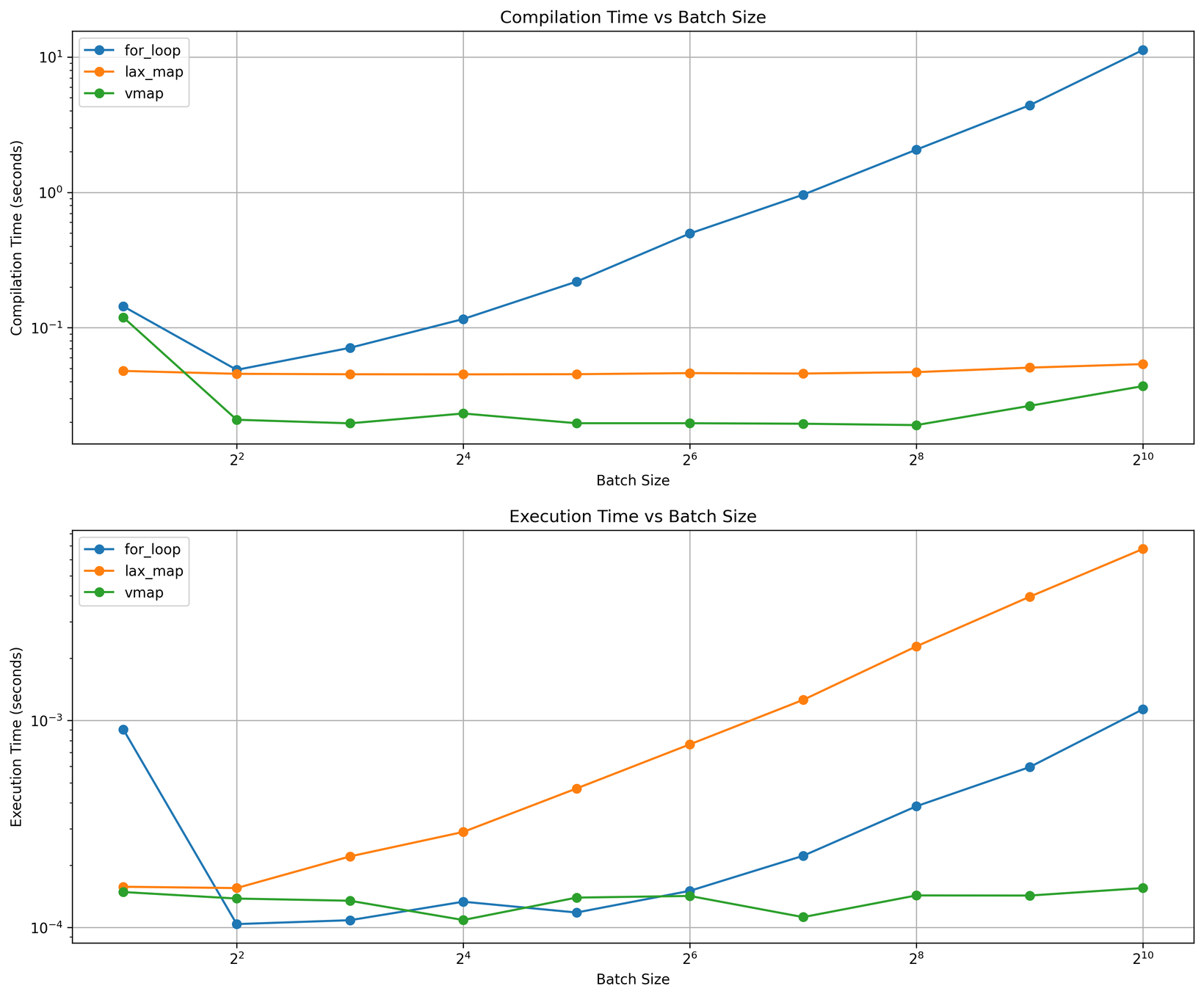
for loops, jax.lax.map, and vmap .In terms of compilation time, we find:
- The compilation overhead grows linearly for
forloops - each iteration added to the sequence demands additional processing time (a direct consequence of loop unrolling). lax.mapmaintains near-constant compilation times across batch sizes (essentially, the ‘inner jaxpr’ andscanprimitive stays the same).vmapachieves the fastest compilation via smart broadcasting primitives and a compact representation.
In terms of execution time, we find:
jax.vmapis the most performant.lax.mapis the slowest, and since it is executed sequentially, grows with the number of iterations (batch size).- The
forloop is faster thanlax.mapand slower thanjax.vmap, with execution time growing sub-linearly with batch size. This can be attributed to XLA's ability to fuse operations (see next section) between unrolled iterations, partially mitigating the overhead of loop expansion.
With this, we can make informed decisions: standard Python loops suit small fixed-size batches but suffer from slower compilation and execution due to lack of vectorization, while jax.lax.map offers batch size flexibility and efficient compilation despite sequential processing. jax.vmap delivers the fastest compilation and execution via vectorization but demands more memory and may require recompilation with batch size changes. Choose Python loops for simplicity, lax.map for memory constraints, and vmap for performance.
High Level Operations: Deciphering XLA's Computational Blueprint
While jaxprs serves as JAX's intermediate representation, High Level Operations (HLO) serves as XLA's intermediate representation. HLO sits between jaxprs and the final machine code, providing a platform for hardware-independent optimizations.
Specifically, HLO represents computations as a graph of operations on statically-shaped arrays. XLA then takes this array-level program as input and performs various optimizations, including operation fusion, common subspace elimination (CSE) and layout optimizations etc. The result produces a compiled binary for a target hardware accelerator.
The optimizations can be illustrated with the following example:
Example: Feed Forward Layer
One of the key optimizations performed by XLA on the HLO representation is operation fusion. JAX's original paper provides an example of this for a neural network layer with a non-linearity:
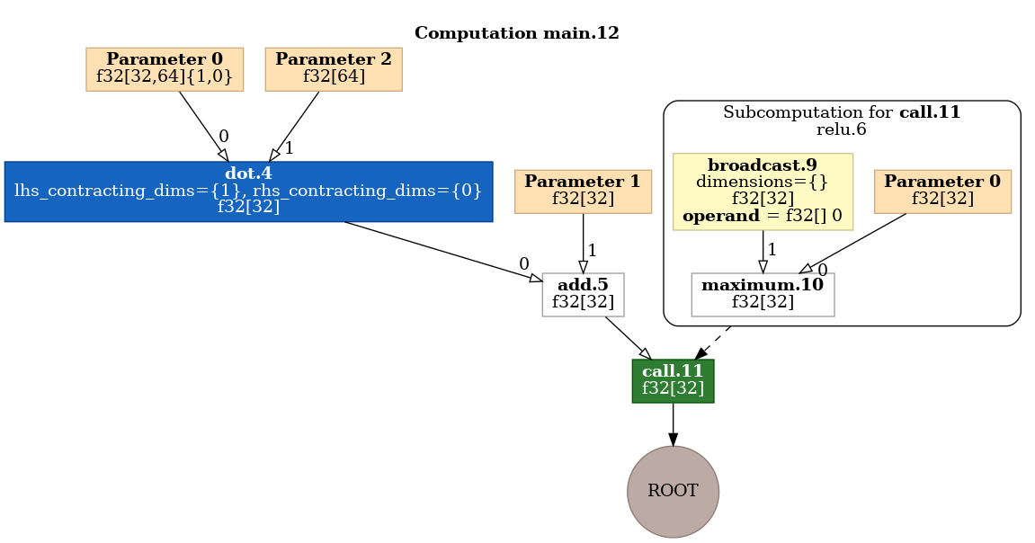
- Initially, the HLO graph contains separate operations for matrix multiplication, addition, and the activation function.
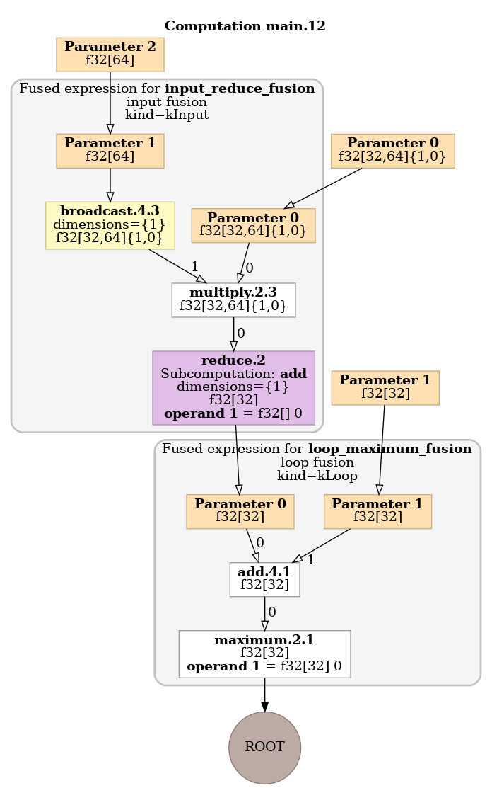
- After optimization, XLA fuses these operations into a single, more efficient operation.
This fusion can lead to significant performance improvements by reducing memory bandwidth usage and enabling more efficient use of hardware resources. Taking our previous layer_forward function, we can see this in action:
Jaxpr Representation
The overall structure of our computation is given by:
jax.make_jaxpr(layer_forward)(params, x){ lambda ; a:f32[32,64] b:f32[32] c:f32[64]. let
d:f32[32] = dot_general[...] a c
e:f32[32] = add d b
f:f32[32] = pjit[name=relu ...] e
in (f,) }Here we see three distinct operations: matrix multiplication (dot_general), addition, and the ReLU activation function.
Unoptimized HLO Representation
The unoptimized HLO maintains this separation of operations:
jax.jit(layer_forward).lower(params, x).compiler_ir('hlo').as_hlo_text()ENTRY main.16 {
Arg_0.1 = f32[32,64]{1,0} parameter(0)
Arg_2.3 = f32[64]{0} parameter(2)
dot.4 = f32[32]{0} dot(Arg_0.1, Arg_2.3), lhs_contracting_dims={1}, rhs_contracting_dims={0}
Arg_1.2 = f32[32]{0} parameter(1)
add.5 = f32[32]{0} add(dot.4, Arg_1.2)
ROOT call.15 = f32[32]{0} call(add.5), to_apply=relu.6 }The ReLU activation is implemented as a separate function relu.6, which is called after the matrix multiplication and addition operations.
Optimized HLO Representation
In the optimized HLO, we see fusion of operations:
jax.jit(layer_forward).lower(params, x).compile().as_text()ENTRY %main.16 (Arg_0.1.0: f32[32,64], Arg_1.2.0: f32[32], Arg_2.3.0: f32[64]) -> f32[32] {
%Arg_2.3.0 = f32[64]{0} parameter(2)
%Arg_1.2.0 = f32[32]{0} parameter(1)
%Arg_0.1.0 = f32[32,64]{1,0} parameter(0)
%input_reduce_fusion = f32[32]{0} fusion(...), kind=kInput, calls=%fused_reduce
ROOT %loop_multiply_fusion = f32[32]{0} fusion(...), kind=kLoop, calls=%fused_multiply
}In this version, operations are fused into two main computations:
fused_reduce: Combines the matrix multiplication (dot product) operation.fused_multiply: Fuses the addition operation with the entire ReLU activation function.
Fused operations can keep data in cache longer, reducing cache misses.
Graphical Representation
We can visualize the computational graph of the unoptimized and optimized HLO representations with the following helper functions:
 def todotgraph(x):
    return xla_client._xla.hlo_module_to_dot_graph(xla_client._xla.hlo_module_from_text(x))

def visualize_hlo(hlo_text, filename, output_dir):
    os.makedirs(output_dir, exist_ok=True)

    # Write HLO text to file
    with open(os.path.join(output_dir, f"{filename}.hlo"), "w") as f:
        f.write(hlo_text)

    # Convert HLO to dot graph
    dot_graph = todotgraph(hlo_text)

    # Write dot graph to file
    with open(os.path.join(output_dir, f"{filename}.dot"), "w") as f:
        f.write(dot_graph)

    # Convert dot file to PNG
    os.system(
        f"dot {os.path.join(output_dir, filename + '.dot')} -Tpng > {os.path.join(output_dir, filename + '.png')}")
For the unoptimized HLO, the output illustrates the separated computations:
For the optimized HLO, the output illustrates the two fusion blocks:
Remarks
When encountering slow compilation times in JAX, investigating the HLO representations can reveal potential optimization opportunities. Key points to consider include:
- Using flags to dump HLOs to text files during compilation, for example:
XLA_FLAGS="--xla_dump_hlo_as_text --xla_dump_to=xla_dump python your_script.py. The text files can then be examined for any suspiciously outsized HLOs. For example, pay attention to unexpected repeated structures (see this git issue as a case study) - For simpler computations, visuals of HLO dot graphs may help locate duplicate operations, identify excessive broadcasting, or find opportunities for fusion.
Profiling: Digging into More Complex Programs
Armed with an understanding of XLA, we can more confidently approach advanced profiling tools when dealing with more complex programs. Without this knowledge, it can be overwhelming to interpret stack trace flamegraphs and diagnose performance issues effectively.
Visual Analysis
JAX offers a built-in profiler that can be visualized using Perfetto. It can be used to generate detailed timeline views of JAX operations, XLA compilations, and hardware-specific kernels, allowing us to identify performance bottlenecks.
For larger programs, tracking the computational flow can get messy. Annotating functions can be useful for decoding and visually stamping specific operations in the trace visualization, making it easier to understand the high-level structure of the program's execution. To illustrate this concept, consider a simulation with various modular functional components running in a loop, (here, we deal with a simple lattice Boltzmann simulation for fluid flow). We can @annotate_function individual functions and use TraceAnnotation for different phases of our program:
@annotate_function
@jax.jit
def macroscopic(fin, v):
    ...

@annotate_function
@jax.jit
def equilibrium(rho, u, v, t):
    ...

@annotate_function
def inivel(uLB, ly):
    ...

@annotate_function
@jax.jit
def apply_outflow_boundary(fin, col_2):
    ...

@annotate_function
@jax.jit
def compute_rho_u(fin, v, vel, col_1, col_2):
    ...

@annotate_function
@jax.jit
def apply_inlet_boundary(fin, feq, col_0, col_2):
    ...

@annotate_function
@jax.jit
def collide(fin, feq, omega):
    ...

@annotate_function
@jax.jit
def bounce_back(fout, fin, obstacle):
    ...

@annotate_function
@jax.jit
def stream(fout, v):
    ...

@annotate_function
def timestep(fin, vel, obstacle, col_0, col_1, col_2, nx, ny, v, t, omega):
    fin = apply_outflow_boundary(fin, col_2)
    rho, u = compute_rho_u(fin, v, vel, col_1, col_2)
    feq = equilibrium(rho, u, v, t)
    fin = apply_inlet_boundary(fin, feq, col_0, col_2)
    fout = collide(fin, feq, omega)
    fout = bounce_back(fout, fin, obstacle)
    fin = stream(fout, v)
    return fin, rho, u

with jax.profiler.trace("./simulation_profiling_output/trace", create_perfetto_link=True):
    with TraceAnnotation("Main Loop"):
        for time in range(maxIter):
            with TraceAnnotation("Timestep"):
                fin, rho, u = timestep(fin, vel, obstacle, col_0, col_1, col_2, nx, ny, v, t, omega)
In this scenario, annotations would allow us to distinguish different phases of the simulation, such as time-stepping, collision, streaming, and boundary conditions:

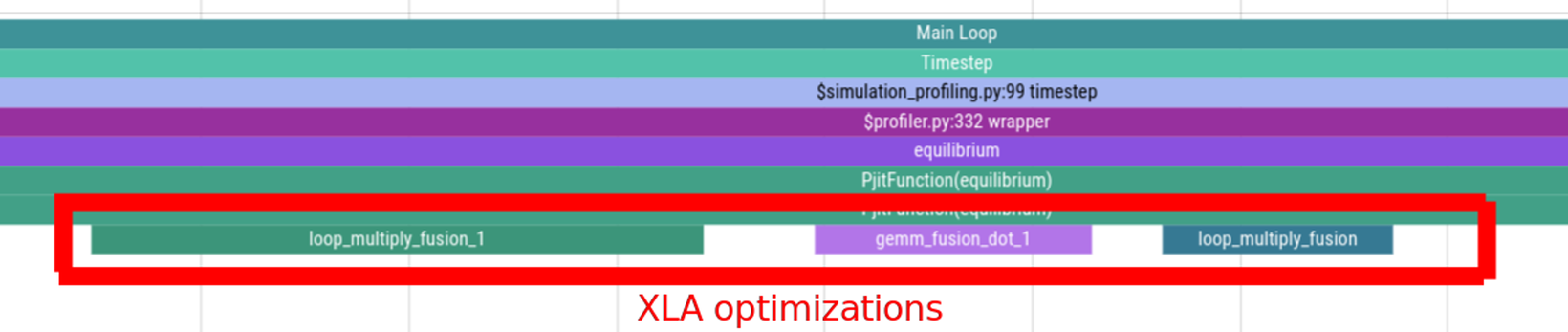
We can zoom in to functions of interest and identify their XLA optimizations and corresponding compilation and execution times (when using JIT, remember the function compiles on its first run). For example, we can verify if our code is being properly vectorized and if operations are being fused as expected:
For GPU-accelerated code, we can see individual kernel launches and their duration, helping identify potential GPU under-utilization or kernel inefficiencies:

In general, when analyzing the Perfetto trace, we can pay attention to:
- Repeated patterns: In our simulation loop, look for consistent timings across iterations, which indicate stable performance.
- Unexpected delays: Long gaps between kernel executions might indicate CPU-GPU synchronization issues or underutilization.
- Compilation spikes: Large spikes in execution time, especially early in the trace, often indicate JIT compilation. Ensure these only happen once per function unless you're expecting recompilation.
- Balance between stages: In our simulation, check if certain stages (e.g., collision or streaming) are disproportionately slow, indicating potential optimization targets.
Quantitative Analysis
Trace data in Perfetto is stored in a highly structured format, allowing for efficient querying and analysis. The TraceProcessor class provided by the Perfetto library effectively transforms trace data into queryable databases. This approach enables us to execute SQL queries, providing a flexible and efficient means of extracting specific information without the need to load the entire trace into memory.
For instance, we can create a helper function that performs SQL querying to extract key performance metrics:
import gzip
from perfetto.trace_processor import TraceProcessor

def analyze_trace(trace_path, annotation_name):
    with gzip.open(trace_path, 'rb') as trace_file:
        tp = TraceProcessor(trace_file)
        # Find instances of the annotated function
        query = f"""
            SELECT ts, dur
            FROM slices
            WHERE name = '{annotation_name}'
            ORDER BY ts
        """
        result = tp.query(query)
        df = result.as_pandas_dataframe()
        if not df.empty:
            num_calls = len(df)
            # It compiles on the first run
            compile_time = df['dur'].iloc[0]
            if num_calls > 1:
                # Average duration of subsequent runs
                avg_execution_time = df['dur'].iloc[1:].mean()
            else:
                avg_execution_time = 0
            metrics = {
                'Metric': ['Compile Time (ms)', 'Average Execution Time (ms)', 'Number of Calls'],
                'Value': [compile_time / 1e6, avg_execution_time / 1e6, num_calls]
            }
            print(metrics)
            return compile_time, avg_execution_time, num_calls
        else:
            print(f"No instances of the annotation '{annotation_name}' found in the trace.")
            return None, None, 0
Here, we select the start time (ts) and duration (dur) of each slice (a span of time in the trace) that matches a specified annotation name, allowing us to get the compilation overhead and runtime performance of specific JIT-compiled functions.
Executing this function might yield results like:
path = "./trace/plugins/profile/2024_08_21_09_30_36/perfetto_trace.json.gz"
name = "equilibrium"
compile_time, avg_execution_time, num_calls = analyze_trace(trace_path=path, annotation_name=name)
{'Metric': ['Compile Time (ms)', 'Average Execution Time (ms)', 'Number of Calls'], 'Value': [107.060694, 0.04096036833333333, 601]}However, the trace file contains a wealth of information beyond what this query extracts. Various tables and schemas within the trace data can be explored for more advanced analytics. For instance:
- Event types: Query the
slicestable to see all types of events recorded. - Thread and process information: Examine the
thread_trackandprocess_tracktables to understand the execution context of different operations. - Counter events: The
counter_trackandcountertables can provide insights into changing values over time, such as memory usage. - Flow events: The
flowtable can help visualize dependencies between different operations.
By designing more complex queries, we can dive deeper into specific aspects of our program's performance. For example, we might want to analyze the distribution of execution times, identify patterns in memory usage, or track the flow of data between different parts of our program.
Concluding remarks
JAX's design philosophy is purposefully high level, making clear distinctions as to what is left to the developer (code semantics), and what is left to the compiler (optimizations). This approach enables powerful automated optimizations through XLA that would be impractical to achieve manually for non-domain experts. However, having an understanding of both worlds allows us to design algorithms that align with JAX's optimization strategies, write code that's amenable to compiler optimizations, and use profiling tools effectively to address performance bottlenecks.
While the high-level approach might initially seem restrictive to HPC engineers and the low-level intricacies daunting for general users, I hope this article convinces both sides the value of working in the middle ground.
References
JAX’s Autodidax Documentation: JAX’s minimalist autodiff library for educational insights into forward and reverse mode autodiff principles (JAX Docs).
MLSYS 2018 JAX Paper: Foundational paper on JAX's design, enabling high-performance, scalable autodiff for ML on accelerators (MLSYS 2018).
SC-W 2023 Paper Comparing JAX and OpenMP: Examining JAX as high level GPU code (SC-W 2023).
How does it work?: A post by Marie-Hélène Burle with a helpful visual of JAX’s execution pipeline (Blog Post).
Stack Overflow on lax.map vs. vmap: Discussion on the tradeoffs in memory and performance between jax.lax.map and jax.vmap (Stack Overflow).
Visualizing the computational graph of a JAX program: A post by Bojan Nikokic visualizing HLO (Blog Post).
Contributors
This article was written by Thomas Ghorbanian and reviewed by Ivo Timoteo and Guido Cossu.