Taking derivatives with respect to shapes, à la Hadamard. Braid Notebooks

Introduction: finding optimal designs

At Braid we are developing technologies to automate the design of high performance devices and this often translates into algorithms finding a shape that is, under certain criteria, considered optimal.

What does “optimal” mean here? This is best illustrated by an example.

Suppose you want to design a hook, i.e. an object which will be attached to an axis and which must be able to carry a specific maximum load. However, there is a catch: you want this object to be as light as possible.

We can make the problem of finding the "best” design for this hook more precise by stating that:

It must minimize the amount of material used for its fabrication…
… while withstanding the specified load requirements…
… while respecting safety constraints on maximum stresses and strains…
… and, of course, respecting the laws of physics!

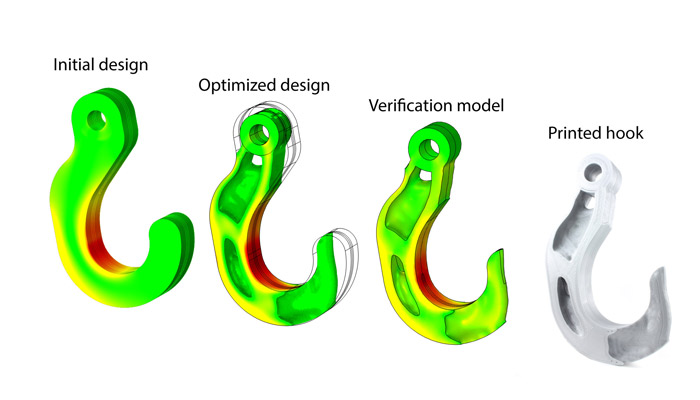
Figure 1: Example of the topology optimization workflow. From this article.

The optimization procedure may consider various parameter classes, from just a few sizes of the object (like width or length) to the entire distribution of material anywhere in space. The corresponding optimization problems are typically called, sizing optimization, shape optimization or topology optimization — if we allow the object to gain new holes.

The final designs for the last two classes are often very organic-looking, and different from the Engineering designs constrained by the classic CAD tools:

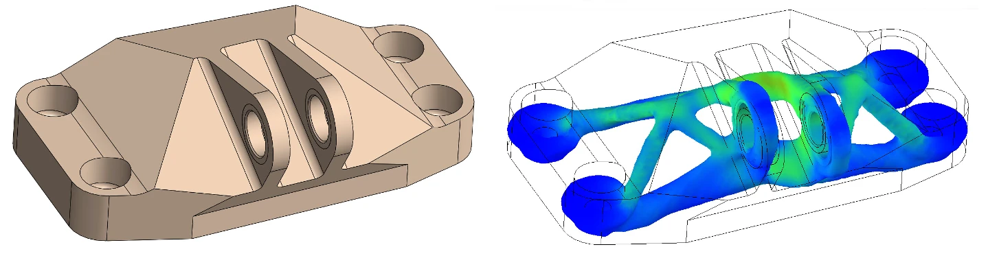
Figure 2: Input and output of topology optimization process. Adapted from here.

The theories behind shape and topology optimization are fairly recent in the history of mathematics, and something that folks with a background in math or physics might find interesting. Our goal in this post is to share the basics of those theories with you.

Optimization (often) means calculating gradients

If you have taken a Calculus class, you might remember that finding maxima and minima of a single valued function requires us to compute its derivatives, and find the points where these derivatives equal zero.

Calculating derivatives — or gradients, as they are called in higher dimensions — is the key behind many optimization algorithms, for instance, the simple gradient descent algorithm: if we are given a function \(f(x)\) which takes a vector argument \(x\), then the process of minimizing \(f\) consists of sequential updates of the form

x_{n+1,i}=x_{n,i}-\alpha \left. \frac{\partial f}{\partial x_i}\right|_{x = x_n},\quad n=1,2,\ldots

where \(\alpha\) is a positive real, the index \(i\) represents the component of \(x\), and \(n\) represents the iteration step in the optimization procedure. We see that being able to compute the derivatives \(\partial f/\partial x_i\) is key for the algorithm to work.

In our design problem, we have an objective function \(J\) (for example, the total mass of our object, or the inverse of its stiffness) which depends on the shape of the object. We want to find the best shape in order to minimize this quantity. Informally, what we would love to do is something analogous to

\text{shape}_{n+1}= \text{shape}_n-\left.\alpha \frac{\partial J}{\partial \text{shape}}\right|_{\text{shape}=\text{shape}_n}

But does it even make sense to compute the derivative of something with respect to a shape?

In 1908, the French mathematician Jacques Hadamard decided that it did make sense, and formulated it rigorously — let’s dive into it.

Figure 3: A photograph of the memoir presented by Hadamard in 1908. From [1].

The Hadamard shape derivative

Hadamard's construction requires three ingredients:

A domain \(\Omega\) in \(\mathbb R^n\): our shape is the boundary of this domain;
A functional \(J(\Omega)\), i.e. a function which takes in the shape domain as an argument and returns a real number. This is the function that we want to minimize.
- A “function of the domain” might sound abstract, but it really isn't: a simple example is \(J(\Omega)=\mathrm{Volume}(\Omega)\) which computes the volume of the region; another one could be the energy contained in the electromagnetic field in a region of space.
A vector field \(\boldsymbol\theta\), i.e. a function \(\boldsymbol\theta(x)\) that assigns a vector at each point of space. In Hadamard's construction, this vector field must be "small" in a very precise sense; but for now the intuition of it is that it will move every point in space to a nearby point via

x \rightarrow x+\boldsymbol\theta(x)

The action of \(\boldsymbol\theta\) on the whole domain \(\Omega\) is to deform it into a new domain \(\Omega_\theta\), which is "close” to the original one.

Illustration of how the boundary of a domain Ω (with Ω being a disk), gets deformed by the action of θ. We only show how the boundary deforms to avoid clutter, but points inside the domain are also mapped to new points inside the new domain. From [1]. — Figure 4: Illustration of how the boundary of a domain \(\Omega\) (with \(\Omega\) being a disk), gets deformed by the action of \(\boldsymbol\theta\). We only show how the boundary deforms to avoid clutter, but points inside the domain are also mapped to new points inside the new domain. From [1].

Illustration of how the boundary of a domain \(\Omega\) (with \(\Omega\) being a disk), gets deformed by the action of \(\boldsymbol\theta\). We only show how the boundary deforms to avoid clutter, but points inside the domain are also mapped to new points inside the new domain. From [1].

Hadamard then argues that there is a natural notion of a shape derivative along \(\boldsymbol\theta\). To see this, first remember the notion of a Taylor series in regular Calculus: one can write, for a general differentiable function \(f\),

f(x+h)=f(x)+f'(x)h+\text{terms in $h^2$, $h^3$ etc.}

We can change our point of view, however, and see this equation as a definition of the derivative \(f'(x)\): it is the expression multiplying the \(h\) term in the expansion of \(f(x+h)\). Although it may sound roundabout, it is a natural way to define derivatives in more complex situations, in particular Fréchet derivatives — and this is exactly what we do now.

We repeat this process for shape derivatives: if we can expand the function \(J\) calculated on \(\Omega_\theta\) as something along the lines of

J(\Omega_\theta)=J(\Omega)+\text{linear form}(\boldsymbol\theta)+ \text{other terms}

such that the “other terms” go to zero faster than \(\boldsymbol\theta\) itself as \(\boldsymbol\theta\) goes to zero, then this "linear term” is our shape derivative. More precisely, if we have

\boxed{J(\Omega_\theta)=J(\Omega)+DJ(\Omega)(\boldsymbol\theta)+o(\boldsymbol\theta),\quad \text{where} \; |o(\boldsymbol\theta)|/\|\boldsymbol\theta\| \to 0 \text{ as }\boldsymbol\theta\to 0}

then we call \(DJ(\Omega)\) is our shape derivative.

A more useful form

In practice, we can write exact expressions for the shape derivatives which we can then plug-and-play in applications.

Assume we can write the functional \(J\) as

J(\Omega)=\int_\Omega f(x) dx

where \(dx\) is the volume element in \(\mathbb R^n\). Then, for a broad set of such \(f\)'s, we can write the shape derivative along a vector field \(\boldsymbol\theta\) as either a volume integral or a surface integral:

\boxed{DJ(\Omega)(\boldsymbol\theta)=\int_\Omega \mathrm{div}(f\boldsymbol\theta)dx=\int_{\partial\Omega}f\;\boldsymbol\theta\cdot \mathbf{n}\,d\sigma}

where, in the second equality, we used the divergence theorem: \(\mathbf{n}\) is the unit normal to the boundary \(\partial\Omega\), which is assumed regular enough for the theorem to hold.

We are just presenting the results here without proof; I highly recommend checking the lecture notes in [1] for proofs and more precise statements.

An analogous expression exists for functionals defined on surfaces instead of volumes; but for now let's focus on this (already pretty broad) class of functionals.

Notice how:

The variation depends on \(\boldsymbol\theta\cdot \mathbf{n}\); any component of the vector field \(\boldsymbol\theta\) which is normal to \(\mathbf{n}\) (hence tangent to the surface \(\partial\Omega\)) won't contribute to the shape derivative at all — they are higher-order terms, which the shape derivative, a first-order quantity, doesn't capture;
Although we are moving the whole domain, the variation of the functional \(J\) can be fully computed by an integral happening on the boundary of \(\Omega\).

A first example: variation of volume

The simplest example we can consider is the volume functional:

J(\Omega)=\mathrm{Vol}(\Omega)=\int_\Omega 1dx.

Then, we can compute the shape derivative of volume as

D\mathrm{Vol}(\Omega)(\boldsymbol\theta)=\int_{\partial\Omega} \boldsymbol\theta\cdot \mathbf{n}\,d\sigma.

To make the example more concrete, assume we are in \(\mathbb R^3\) and let \(\Omega\) be the ball with radius \(R\) centered on the origin. Then we know that \(\mathbf{n} = \mathbf e_r\) is the radial unit vector. Then, in spherical coordinates \((r,\Theta,\varphi)\) (we are using a capital Theta to avoid confusion with the vector field \(\boldsymbol\theta\)) we have

D\mathrm{Vol}(\Omega)(\boldsymbol\theta)=R^2\int_0^\pi \sin\Theta d\Theta\int_0^{2\pi}d\varphi \; \theta_r(R,\Theta,\varphi)

where \(\theta_r\) is the radial component of \(\boldsymbol\theta\). If, for simplicity, we take it as a constant over the 2-sphere, then we get

D\mathrm{Vol}(\Omega)(\boldsymbol\theta)=4\pi R^2 \theta_r(R)

and we find the intuitive result that, if \(\theta_r\) is positive, the volume will increase; analogously, if negative, volume decreases.

A more complex example: moments of inertia

We will illustrate the usage of shape derivatives in a physics problem: that of calculating the moment of inertia of a rigid body. This quantity, denoted as \(I\), measures how hard it is to rotate the body around a chosen axis of rotation. For a body occupying a volume \(\Omega\), the moment of inertia around a rotation axis \(z\), is

I(\Omega)=\int_\Omega \rho \,r^ 2\,dV

where \(\rho\) is its density and \(r\) is the distance from a point to the rotation axis; in usual Cartesian coordinates, if we fix the \(z\) axis as our rotation axis, then \(r^2=x^2+y^2\).

Consider a cylinder with radius \(R\) and height \(L\), with mass density \(\rho_0\):

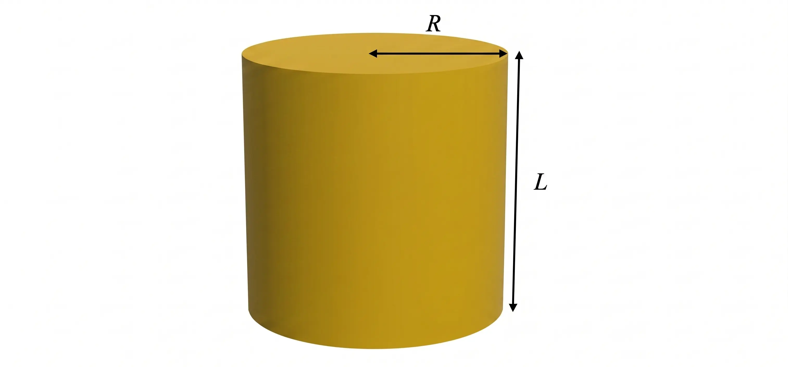
It is not difficult to show that its moment of inertia around the vertical axis passing through the center of the cylinder is

I_0=\frac{\rho_0 \pi}{2}R^4L.

This quantity can also be written as

I = \frac 12 MR^2

where \(M \equiv \pi R^ 2 L \rho_0\) is its total mass. Both forms will be useful in what follows.

We could perform this calculation analytically since there is a high degree of symmetry; it won’t be the case for any general shape.

Now, one might ask: how would the moment of inertia change if we perturb the cylinder’s shape? Namely, what if we make it cave inwards like this:

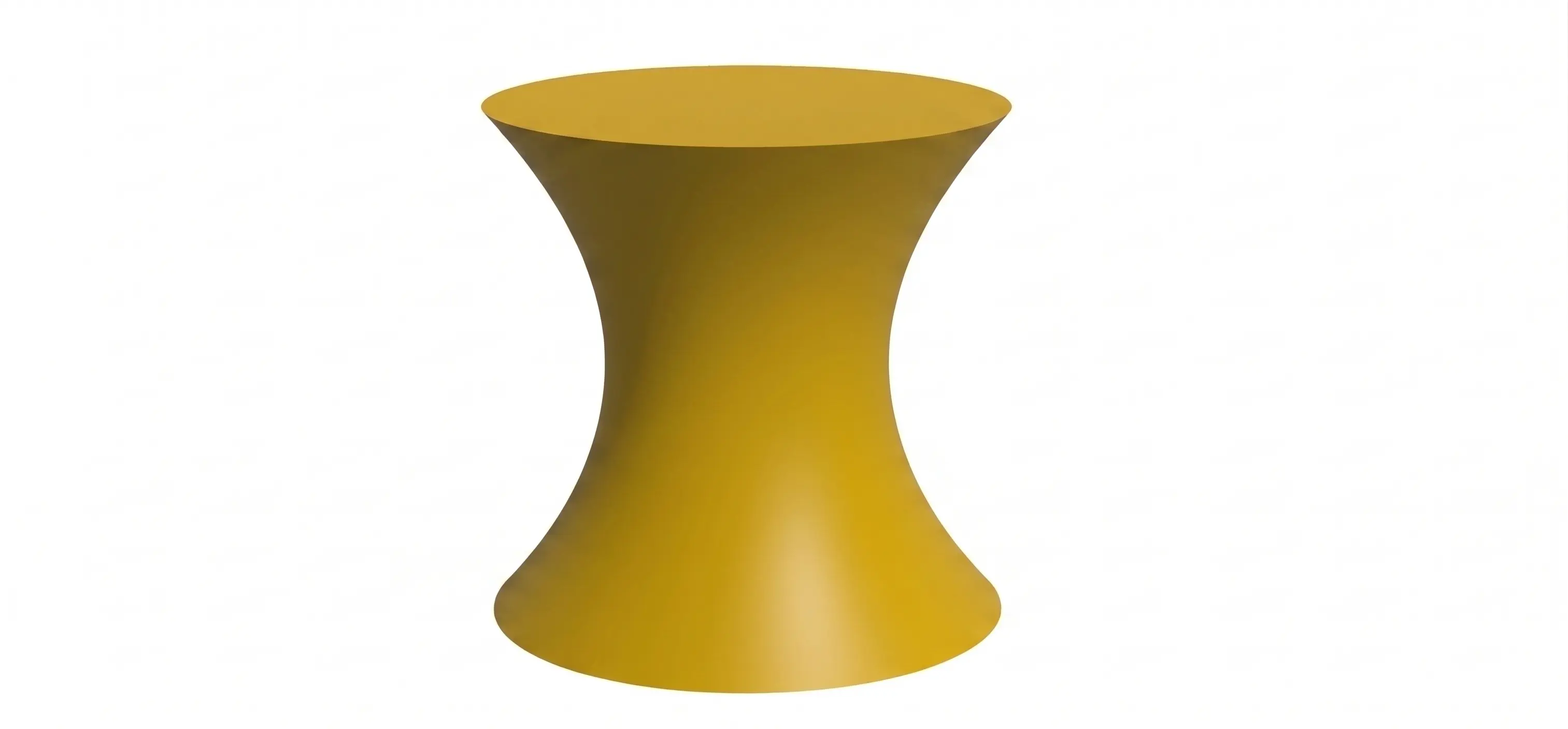
Figure 6: Exaggerated example of the deformation of the cylinder. In practice this would be much more discreet.

Intuitively, we know that the new moment of inertia will be smaller than the original one — in general, for a fixed amount of mass, moments of inertia are smaller for bodies which are more compact in the direction perpendicular to the axis of rotation.

Let’s model the cylinder’s new shape by redefining its radius to be a function of \(z\), namely

r(z)=R-\alpha \frac{z(L-z)}{L}

where we set \(\alpha\) as a small numerical constant, i.e. we assume \(\alpha \ll 1\), and compute everything to order \(\alpha\) excluding order 2 or higher terms.

We can calculate the new moment of inertia in two ways:

From the definition: we calculate the moment of inertia from scratch
Using the Hadamard shape derivative

Below, we illustrate both approaches.

1. From the definition

A trick to accelerate our computation of the moment of inertia is to consider the new “cylinder” as a large collection of smaller cylinders, each with radius \(r(z)\) and mass \(dm\).

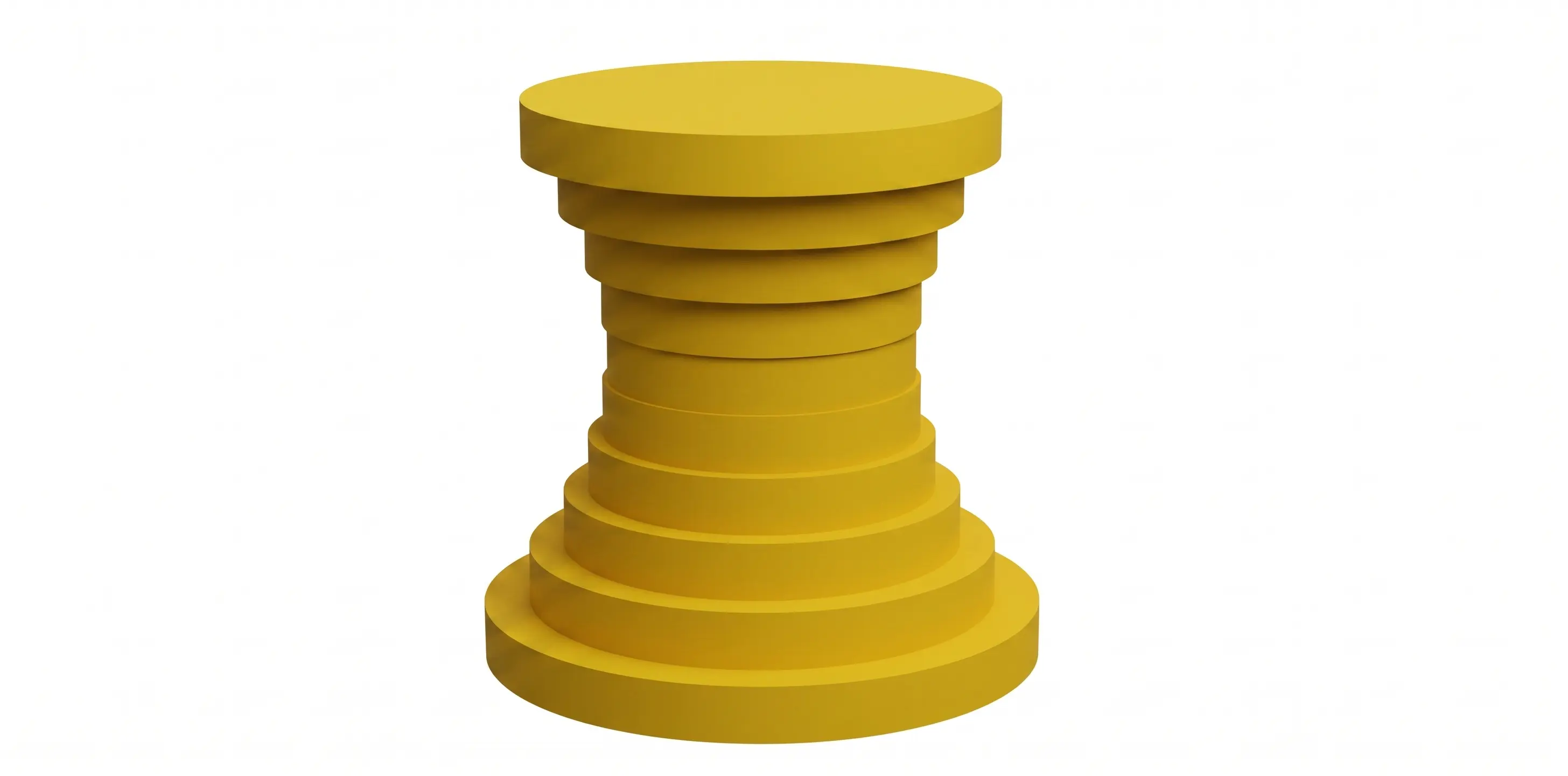
Figure 7: Illustration of the cylinder being considered as a stacked collection of smaller cylinders.

Above, we concluded that a cylinder has moment of inertia \((1/2) MR^ 2\); this means that each infinitesimal cylinder will have a moment of inertia \((1/2) r^2(z) dm\), and so we can write the total moment of inertia as

I = \int_{z=0}^{z=L} \frac 12 r^2(z) dm(z)

Since each element is a cylinder with radius \(r(z)\) and height \(dz\), we may write the \(z\) dependent mass term as \(dm(z) = \rho_0\pi r(z)^2 dz\), and so we must compute the integral

I=\frac{\rho_0 \pi}{2} \int_0^L r^ 4(z)dz=\frac{\rho_0 \pi}{2} \int_0^L \left[R-\alpha \frac{z(L-z)}{L} \right]^4 dz

Since we assumed \(\alpha \ll 1\), we may Taylor expand the integrand to first order in \(\alpha\) and ignore the other terms . The integral then yields

I=\frac{\rho_0 \pi}{2} \int_0^L \left[R-\alpha \frac{z(L-z)}{L} \right]^4 dz =\frac{\rho_0 \pi L}{2}\left(R^ 4 - \frac{2}{3} \alpha LR^3\right) + O(\alpha^2),

and by comparison with the expression for the original moment of inertia \(I_0\), we realize we can simplify this as

I=I_0\left(1-\frac 23 \frac{\alpha L}{R}\right).

Indeed, this quantity is smaller than \(I_0\), as expected.

2. From the shape derivative

We introduce a perturbation in the radial direction (tangent to the \((x,y)\) plane) as

\boldsymbol \theta=-\alpha \frac{z(L-z)}{L} \mathbf e_r.

Then, noting that the moment of inertia can be written as

I(\Omega)=\int_\Omega f\,dV,\quad f\equiv \rho_0 (x^2+y^2)

we can immediately write the shape derivative of \(I\) along \(\boldsymbol \theta\) as

DI(\Omega)(\boldsymbol\theta)=\int_{\partial\Omega}f\,\boldsymbol\theta \cdot \mathbf n\,d\sigma

Since \(\Omega\) is a cylinder, an integral over the boundary is of the form

\int_{\partial\Omega}=\int_\text{side wall}+\int_\text{top}+\int_\text{bottom};

notice, however, that \(\boldsymbol\theta\) only has a radial component whereas the top and bottom surfaces are oriented along the \(z\) axis; since the integrals contain the projection of \(\boldsymbol\theta\) along the normal \(n\), it follows that the two last integrals vanish and we may compute only that over the side wall, namely

\begin{align*}\int_\text{side wall}f\,\boldsymbol\theta \cdot \mathbf n\,d\sigma &= \int Rd\varphi dz\;\rho_0 \underbrace{(x^2+y^2)}_{=R^2}\; \left[-\alpha \frac{z(L-z)}{L} \right]\\ &= -2\pi\rho_0R^3 \int_0^L\frac{z(L-z)}{L} dz\\ &=-2\pi\rho_0R^3 \frac{L^2}{6}\\ &=-\left(\frac{\rho_0 \pi}{2} R^4L\right) \alpha \frac{2L}{3R}\\ &=-I_0 \cdot\alpha\frac{2L}{3R}. \end{align*}

The new moment of inertia will then be the old one plus this small change:

\begin{align*} I &=I_0+DI(\Omega)(\boldsymbol\theta)\\ &=I_0-I_0 \cdot\alpha\frac{2L}{3R}\\ &=I_0\left(1-\frac{2\alpha L}{3R}\right) \end{align*}

which is exactly the same result as that of the exact calculation (when taken to first order). We can argue that this result is relatively simple to compute since \(\boldsymbol\theta\) appears linearly inside the integral; in the general case, like in the example above, it can appear in many ways —there it was raised to the 4th power — and it was up to us to Taylor expand in order to impose the smallness of the perturbation.

Outlook and limitations of this method

Shape derivatives have a natural limitation in that they only provide us ways to create small deformations of shapes. In particular, they will never allow us to pinch a shape or make it self-intersect; in this sense, they are great tools for shape optimization, but not for topology optimization — we will never be able to create holes using this method.

Recently, there has been progress [4] on mixing the use of shape derivatives with the level-set method, [3] the latter being a way of thinking of \(n\)-dimensional shapes as being slices of a shape embedded in \(n+1\) dimensions.

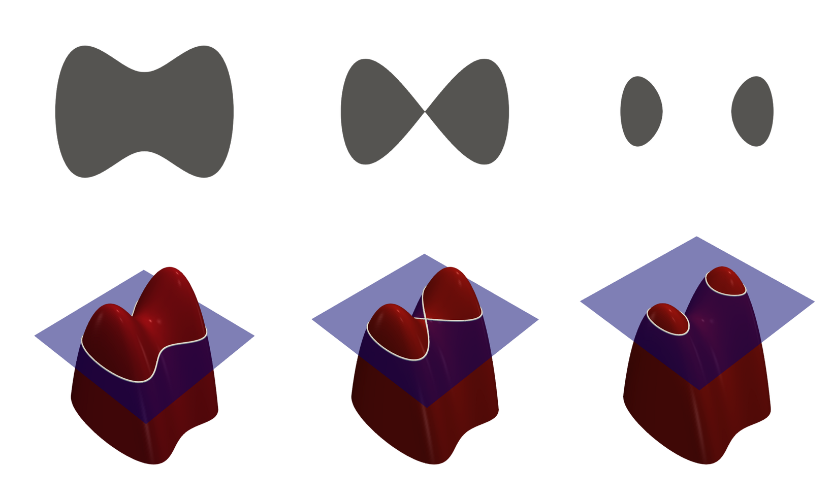
Figure 8: Illustration of a 2D surface seen as a 2D slice of a 3D object. From the Wikipedia page.

Notice that the level-set method naturally allows for topology changes, as the example above illustrates: although the 3D object itself never changes, just by shifting the position of the slicing plane, we get different topologies in 2D.

By mixing the shape derivative with the level-set method, i.e. by taking successive “small displacements” on a higher-dimensional object, we can in fact go beyond shape optimization and do full topology optimization. See references [2] and [3] for more details.

Applying to real-world problems

This is where the things get interesting but also harder. We will give a brief overview of the major concepts but will not go into some of the details.

For topology optimization problems that are relevant to engineering we don’t usually just have a function \(J(\Omega)\) of a domain; its value depends on the solution of a partial differential equation.

To make things more concrete, consider an example. In solid mechanics — used for structural engineering applications — one solves Newton’s second law in order to guarantee that a system remains static. In equations, this is written as

\frac{\partial \sigma_{ab}}{\partial x^b}(\mathbf u)+ \rho g_a=0 \quad \text{on $\Omega$}\quad +\quad \text{boundary conditions on $\partial\Omega$}

where \(\mathbf u\) is a displacement vector which tells us how the system deviates from its rest state under applied loads. The details of this equation don’t matter; all that matters is that the function \(\mathbf u\) which we care about will, indirectly, depend on the domain \(\Omega\). We can write it as \(\mathbf{u = u}_\Omega\).

Now, a common function to minimize is the so-called compliance, a measure of how much elastic energy is contained in the system. It is written as

J(\Omega)=\int_\Omega \sigma_{ab}(\mathbf u_\Omega)\varepsilon_{ab}(\mathbf u_\Omega) dV,

where, again, the details don’t matter — what matters is that this is an integral which depends on \(\Omega\) in two ways: directly as an integration domain, and indirectly through the solution to an equation on \(\Omega\)! This adds a further complication; we can still compute \(DJ(\Omega)\), but we need to further ensure that the physical equations we care about are also satisfied.

This is the perfect scenario for applying so-called adjoint methods; all the formalism we discussed so far still holds, as long as we add the fact that \(\mathbf u_\Omega\) has to solve a physical equation as a constraint (in a Lagrange multiplier kind of setting). Then, shape derivatives can actually be computed — see equation 8 in [2] for a derivation.

Most of engineering problems will require some form of signal provided by the solution of a partial differential equation and generating the derivatives is in principle a tedious and error prone work, but there are multiple techniques to automate the process. As mentioned above, this is a topic that deserves a whole post to itself, so we’ll keep the discussion for another time.

Conclusion

We have discussed how one can take derivatives with respect to shapes in a meaningful manner, as introduced by Hadamard over 100 years ago.

Clearly the mathematics involved is not trivial, especially when we are dealing with physically-constrained problems, as in the structural example above, and when trying to expand our scope to topology optimization. However, it is exactly when we take all these aspects into account that we can find optimal structures for real-world applications.

References

[1] Florian Feppon, lecture notes

[2] Structural optimization using sensitivity analysis and a level set method

[3] The level set method, MIT lectures

[4] Shape and topology optimization, Allaire et al.

Contributors

This article was written by Alessandro Morita and reviewed by Guido Cossu.